

One of the first tasks I did as a part of the Autonomous Ground Vehicle research group was to implement localization and mapping, way back at the end of my first year. I, along with Satyesh and Vasudha (two fellow batchmates), worked right from interfacing the sensors to implementing and testing the algorithms. We did all of this for 2D data and are currently working towards making both localization and mapping work for 3D data.
Localization
One of the most important requirements for automating a robot is its localization. By localization, we mean that the robot must, at all times, have a fairly accurate idea about its position in a given map or environment. If a robot does not know where it is, it can not decide what to do next. In order to localize itself, a robot has to have access to relative and absolute measurements that contain information related to its position. The robot gets this information from its sensors. The sensors give it feedback about its movement and the environment around the robot. Given this information, the robot has to determine its location as accurately as possible. What makes this difficult is the existence of uncertainty in both the movement and the sensing of the robot. The uncertain information needs to be combined in an optimal way. We did so using the Extended Kalman filter algorithm, which is a kind of Bayesian filter.
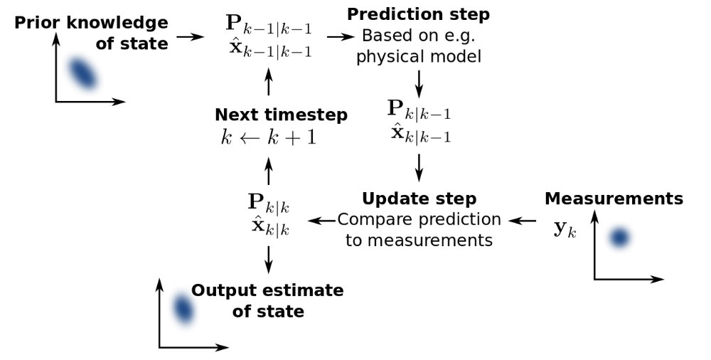
To localize, we used three inputs – odometry data (from wheel encoders), IMU data and GPS data (from Vectornav INS. Since the data received from each of these sensors is inherently noisy, we used the Extended Kalman Filter algorithm. The Extended Kalman Filter is the non-linear version of Kalman Filter which is used widely to produce estimates of unknown variables (linear Gaussian systems) using a Bayes Filter algorithm that uses a series of measurements observed over time (containing noise and other inaccuracies). These measurements tend to be more precise than those based on a single measurement alone. The EKF employs a local linearization using Taylor’s theorem, to employ the Kalman filter algorithm (which uses a linear model) to nonlinear problems.
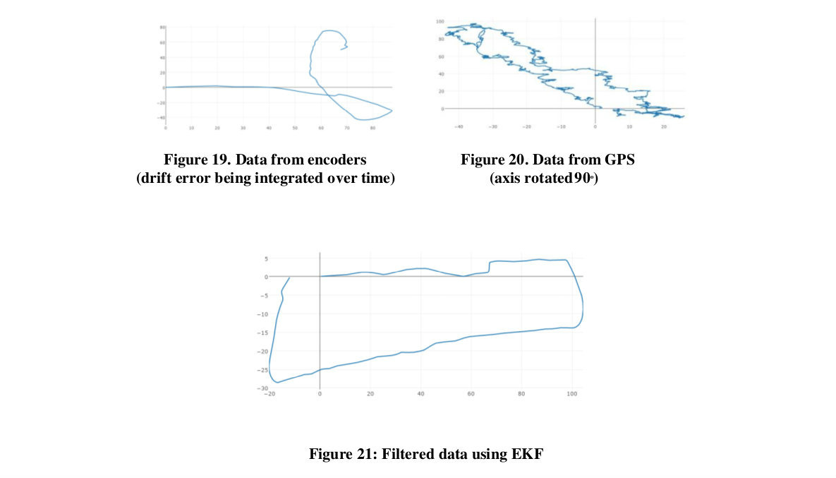
There were problems while integrating GPS data into the filter, especially when the satellite data was inaccurate at some places. In this iteration, the covariance matrices were tuned and an average of 100 iterations of GPS data was used to set the origin in the GPS frame. With this, errors as low as 0.2m (in x and y directions) were achieved after following a closed loop path of perimeter 400m.
Mapping
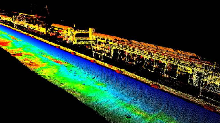
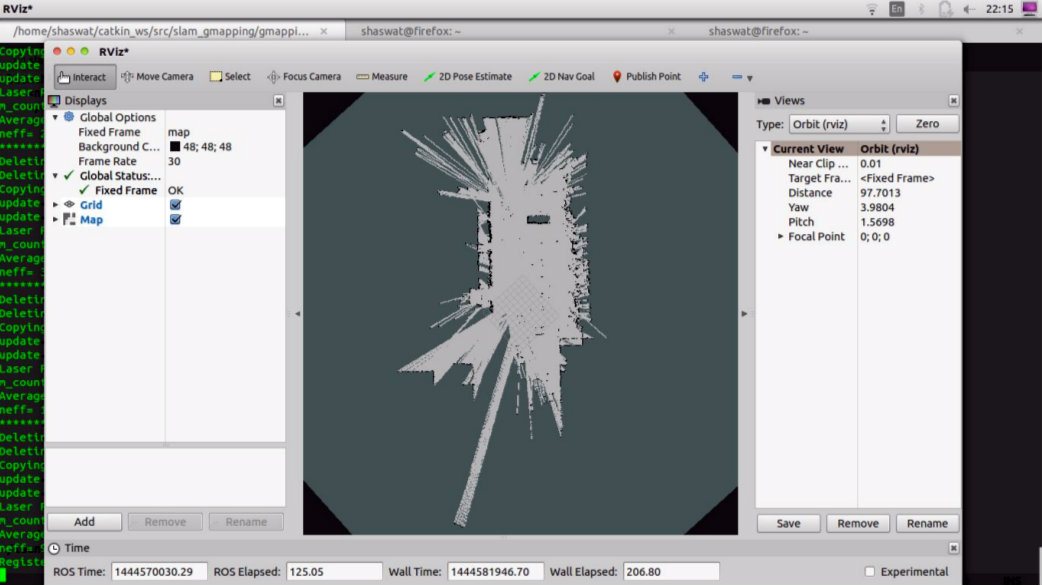
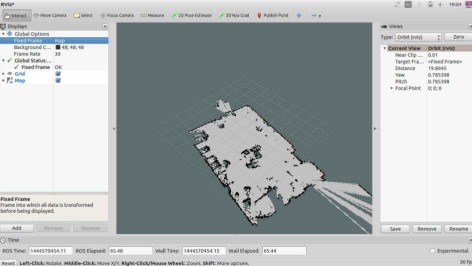
We then fed the filtered odometry data into the GMapping algorithm along with the input from the LIDAR (Laser Scan). GMapping is a highly efficient Rao-Blackwellized particle filter to learn grid maps from laser range data and form a map showing the obstacles around the robot. It uses the filtered odometry data to get the pose of the robot and merges the data with the laser scans received from the LIDAR to produce a map of the robot’s environment. The map of the environment, thus produced is used by our navigation and path planning module.
The map outputs visualized in RViz:
Outdoor Map
Indoor Map
Too many Thanks
Almost perfect guide
Gooⅾ day very nice web site!! Guy .. Beautiful ..
Wonderful .. I will bookmark your web site and taқe the feeds alsⲟ?
I am ѕatisfied to seek out ѕo many useful information here in the post, we need deνelοp more techniquеs in this regard,
thanks for sharing. . . . . .
I like the helpful info you provide in your articles. I’ll bookmark your weblog
and check again here frequently. I’m quite sure I’ll
learn many new stuff right here! Good luck for the next!
generic viagra