

The aim of Safe Reinforcement learning is to create a learning algorithm that is safe while testing as well as during training. The literature on this is limited and to the best of my knowledge, a sample efficient safe RL algorithm is yet to be achieved.
Let’s start with a basic understanding of what we are trying to achieve here:
Safe Reinforcement Learning can be defined as the process of learning policies that maximize the expectation of the return in problems in which it is important to ensure reasonable system performance and/or respect safety constraints during the learning and/or deployment processes.
– Garcia et al 2015
The constraints may be, for example, the case of data-center cooling, temperatures and pressures are to be kept below respective thresholds at all times, or a robot must not exceed limits on velocity, angles and torques; or an autonomous vehicle which must respect its kinematic constraints.
Generally, this problem has been approached in two major ways:
- Change the optimization criteria
- Change the exploration process
Optimization Criteria
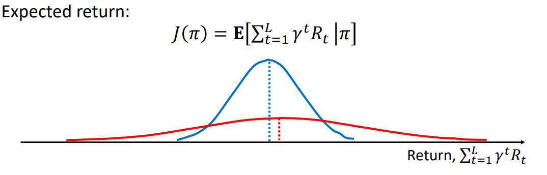
Let J(π) denote the performance of a policy (for now assume it means how good the policy is). Suppose you are in a casino, which policy would you want to follow? The red one or the blue one? The red one! It gives a more expected reward. But suppose the agent is a surgeon, the blue policy works better because it has lesser variance, i.e less chance it will screw up because low rewards are less probable. So, this example suggests that we can consider variance as a one of the measures of risk.
There has been some amount of work to incorporate risk into the optimization objective. Broadly (to keep the blog sane), some methods to do so are:
a. Worst Case Criteria
A policy is considered to be optimal if it has the maximum worst case return. That is, the policy’s worst case reward obtained is maximized. The whole task simplifies to solving the mini-max objective below:
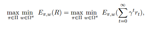
where Ω is a set of trajectories of the form (s0, a0, s1, a1, . . .) that occurs under policy π.
b. Risk-Sensitive Criteria
Include the notion of ‘risk’ in the long term reward maximization objective. Some literature has defined risk as the variance of return. Considering an example of risk sensitivity based on exponential function, a typical objective function can look like:

A taylor expansion of the exp and log term gives us:
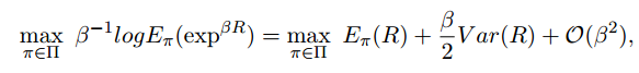
where β denotes the risk-sensitive parameter, with the effect that β being negative aims to reduce the variance in rewards and hence the risk.
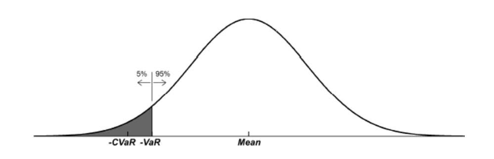
- Some other methods include maximizing Value at Risk (VaR), Conditional Value at Risk (CVaR), or another robust objective. In VaR, we specify a value such the at least 95% (as in the example below) of the times you would get better performance than that value. CVaR is the mean of the worst case returns below VaR (the shaded region). For getting more information about this metric see these answers or the paper.
c. Constrained Criteria
The expectation of return is subjected to one or more constraints. The general form of these constraints is shown below:
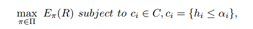
where c_i are the constraints belonging to set C.
Intuitively, for example, a policy is updated if it is safe with a certain confidence given the constraints. I’ll elaborate on the constrained criterion below when I discuss the work of the paper Constrained Policy Optimization.
Exploration Process
Classical exploratory behaviours in RL assume that agent has to explore and learn to weigh different actions and act optimally. Agent ignores the risk of actions, potentially ending in dangerous states. Explorations like the ε-greedy may result in disastrous situations. Also, random exploration policies waste a significant amount of time exploring the regions of the state and action space where optimal policy will never be encountered.
It is impossible to completely avoid undesirable situations in risky environments without external knowledge because the agent needs to visit the dangerous state at least once before labelling it “dangerous”. There can be two ways of modifying the exploration process:
1. Incorporate external knowledge
We can incorporate external knowledge to provide initial knowledge(can be considered as a type of initialization procedure) or derive a policy using a finite set of examples. I’ll elaborate on these techniques below.
Let’s discuss some ways we can provide initial knowledge or do an initialization. In one example we can record a finite set of demonstrations from a human teacher and provide it to a regression algorithm, to build a partial Q-function which can be used to guide further the exploration. These type of methods have also been used in neuroevolution approaches as in (Siebel and Sommer, 2007) whose initialization weights are obtained using a teacher. However, such initialization approaches are not sufficient to prevent dangerous situations which occur in later exploration.
To derive a policy from a finite set of demonstrations, a teacher demonstrates a task and the state-actions trajectories are recorded. All these trajectories are then used to derive a model of the system’s dynamics, and an RL algorithm finds the optimal policy in this model. These techniques fall under the category “Learning from demonstrations”. In this methodology, learners performance is limited by the quality of teacher demonstrations.
2. Risk directed exploration
In this trend, one of the approaches defines a risk metric on the notion of “controllability”. Intuitively, if a particular state (or state-action pair) yields a lot of variability in the temporal-difference error signal, it is less controllable. Controllability of state-action pair is defined as:
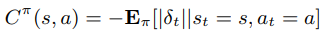
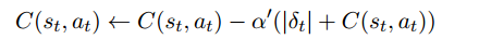
where δ is the temporal-difference error signal. The exploration algorithm seeks to use controllability as an exploration heuristic instead of a general Boltzmann exploration. The agent is encouraged to pick controllable regions of the environment.
Having introduced the classical approaches to safety, I will now move on to the topics which deserve attention, what is yet to be solved and what has been going on in these fields apart from the ideas mentioned above.
We will work on the simple idea of incorporating constraints into the RL agent. It should avoid the things that are ‘risky’ — (definition open to interpretation?) while learning what the agent was made for in the first place.
These constraints we talk about, are being incorporated and research is focused on developing different methods to make this happen. I will classify the type of constraints we are looking to deal with below.
1. Soft constraints
Here, the constraints are not necessarily followed while exploration or sometimes they are followed in expectation.
Example:
2. Hard constraints
The constraints are followed without fail while training and testing.
Example:
- Trial without Error: Towards Safe Reinforcement Learning via Human Intervention
- Safe Exploration in Continuous Action Spaces
Consider a human learning to drive a car. Do you think he/she learns to drive following hard constraints? Or will the constraints as soft as expectation will do? Humans know beforehand the consequences their actions can have. They know the ‘risk’. If they face a situation where they realise that a constraint is going to be violated, they are already equipped with a recovery behaviour in their mind(or are they?). But sometimes even this recovery behaviour may not be sufficient to pull you out of the risky situation. Is the aim of hard-constraint RL algorithm practical? or should we just try to model the human-version of the same? Are we over-estimating the power of machines?
I will summarise some work done in this direction below. If you are looking for just the gist, you are good with reading the first paragraph for each literature description.
1. Constrained Policy Optimisation [Achiam et al. 2017]
This method falls in the realm of constrained optimization that I have described earlier as the constrained criteria. In this paper constrained policy optimization (optimizing the policy following the constraints specified) was solved with a modified trust-region policy gradient. There, the algorithm’s update rule projected the policy to a safe feasibility set in each iteration. For this, they derive the bound between the difference in returns to the average divergence between two policies that is tractable. Under some policy regularity assumptions, it was shown to keep the policy within constraints in expectation.
It is unsuitable for use-cases, where safety must be ensured for all visited states and during training.

Background for the paper:
The theory starts off with an expression given by Kakade et al in the paper Approximately Optimal Approximate Reinforcement Learning.
I will walk through the proof for expressions required in the paper and will try to give an intuitive understanding of what is actually happening. I will try to give the explanation in such a way that anyone with a background in probability and some in RL will be able to understand.
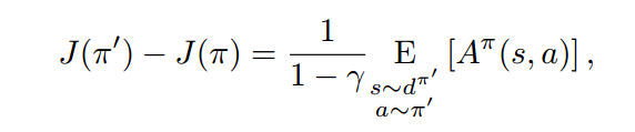
The motivation of the paper is to prove new bounds on the difference
in returns (or constraint returns) between two arbitrary stochastic policies in terms of an average divergence between them. First, let us start with the expression formulated by Kakade et al. This expression says that difference between the performance of two policies is expectation of advantage function for particular state and action in policy π, where the states are sampled from discounted future state distribution of policy π’, and actions from policy π’.
To understand what is really going on here, we will need to be familiar with some notations and preliminary results.
Value function for any policy π is given as:
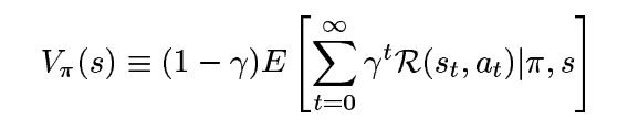
Here, the factor (1-γ) comes from a need to normalize the value function, so that it remains in the range [0-R]. The expectation term is the typical definition. Similarly, Q-function is given as,

and Advantage function is given as,
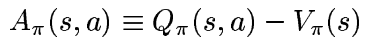
It is easily seen that Q-function lies in [0, R] and A-function lies in [-R, R].
Now we define a new term called the γ-discounted future state distribution. It is imperative to understand what this is, as this is central to formulating the expressions given in the paper.
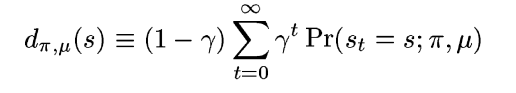
For a starting state distribution μ, the discounted future state distribution is defined as above. (1-γ) term is necessary for normalization. This definition is not totally intuitive and is just whipped up to make it easier for tasks like redefining the value function below. It approximately denotes the probability of visiting a given state while following a policy π with future visitations made less significant through discounting. Now, this definition helps us rewrite the value function defined above as:

Take a moment to think about this. The a’ is sampled from π and s’ from the discounted future state distribution, which indicates the discounted probability that starts at state s and follows policy π. So basically what this equation says is that for every state s’ and state s, it finds a way for each timestep t and multiplies the appropriate reward with the discounted probability of transition happening from s to s’ in time t, for all possible t.
The last relation that we need is what is called the performance of a policy.
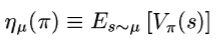
This can be interpreted as given an initial state distribution μ, what is the expected reward that I can get using the policy π. Also, one other interpretation can be the average reward of n episodes for a given policy, with n tending to infinity.
Now, that all the notations are clear let us look at the derivation for the equation we started with as given by Kakade et al.
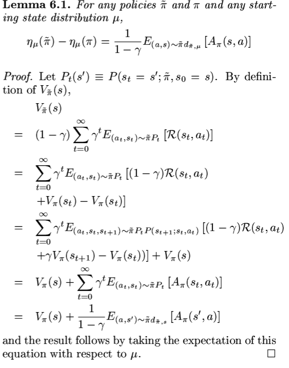
Let’s break down the proof. The first step is clear, it’s the definition of value function. From the second step to the third step, a Value function for state s at time t is broken into the reward that would be obtained from s[t] and the V(s[t+1]) using the policy π. This reward term is pulled out in expectation to give V(s) in policy π.
CPO [Github]
We have the relation the maps the difference in performance of two policy to the expectation of advantage obtained through one policy following another policy.
While this is not practically useful to us (because, when we want to devise a bound with respect to π , it is too expensive to evaluate V(π’) for each candidate to be practical). Also, computing this is a tedious task (because we will need to compute it for every new policy if we are to estimate the performance difference) and we want to relate the difference in performance of policies to the function of the two policies itself. In mathematical terms, we would like our constraints to be in terms of discounted state distribution of current policy(π) only. Acheon et al proves the following bound in the CPO algorithm. Look in the appendix of the paper for the complete proof. (Given the background above, you are equipped to understand the proof on your own)
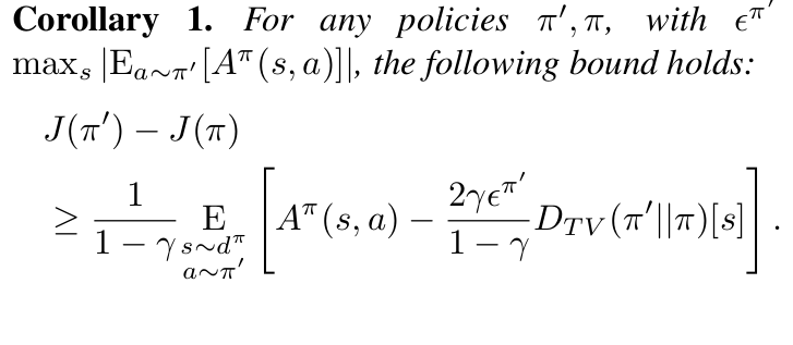
The advantage term with s sampled from d distribution for policy π is an equal to J(π’ ) − J(π) using the state distribution d(π’), which was the first equation we proved . Now using the state distribution d(π) instead of d(π’) , the above bound can therefore be viewed as describing the worst-case approximation error.
2. Safe Exploration in Continuous Action Spaces [Dalal et al. 2018]
This paper is based on learning the policy in presence of hard constraints i.e the constraints should never be violated. In this work, they directly add to the policy a safety layer that analytically solves an action correction formulation per each state. This method largely builds upon the work of OptLayer by T.H.Pham et al.
The method is divided in two sections:
- Linear Safety-Signal Model
The objective of the method is to find finally a parametrized policy such that,
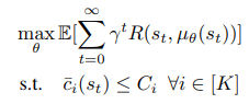
The above equation is equivalent to maximizing the expected reward such that safety signal at each encountered state is less than corresponding constraints on the safety signals. Now, to get the safety signal models beforehand for all states, they learn a function approximator that gives the value of safety signals at each state using a linear approximation.
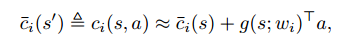
The function g(s;w) is our function approximator here. They learn this using the single step transition data in the logs, solving the following objective.
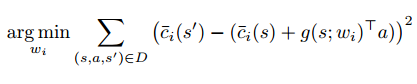
In their experiments, they generate D by initializing the agent in random locations and terminating when the time-limit is reached or in case of constraint violation.
- Safety Layer using Analytical Optimization
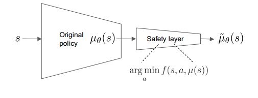
The role of the safety layer is to solve:
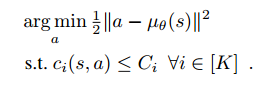
Solving the above equation is equivalent to perturbing the original action as little as possible in Euclidean norm to satisfy the necessary constraints. Substituting the linear safety model we get the quadratic program:
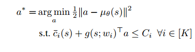
The analytical solution to this equation is found out and this “safe action” is used in training. For example in case of policy gradient methods, instead on the action a, the safe action a* is supplied to the update network call.
Here’s a video of their algorithm running on a toy environment:
3. Off-policy policy evaluation [Precup et al. 2000, P. Thomas 2015]
First of all, the definition of safety is to be changed here. Safety is defined here as with probability atleast 1-δ, the current policy is not changed to a worse policy, where δ represents the probability of choosing a bad policy.
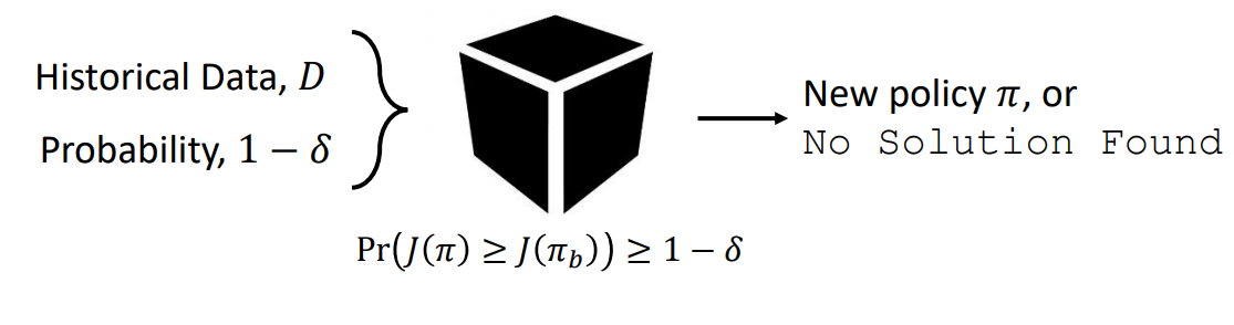
If the policy cannot be improved given the data D, “no solution found” is returned. Note, we are assuming we already have an initial policy. Recent work is going on, how to find this initial policy. Note, here the definition of safety is different
In off-policy policy evaluation we have a behaviour policy π and an evaluation policy π’. We aim to evaluate the performance J(π’) of evaluation policy without deploying π’, as it can be dangerous. Generally, off-policy evaluation refers to predicting value function from policies the did not come from the behaviour policy. Here, we aim to estimate the performance of the new policy, hence the off-policy policy evaluation. The whole aim of the exercise is summarized below:

We will say that the probability that performance of proposed policy is greater than behaviour policy will be atleast 1-δ.
Importance Sampling
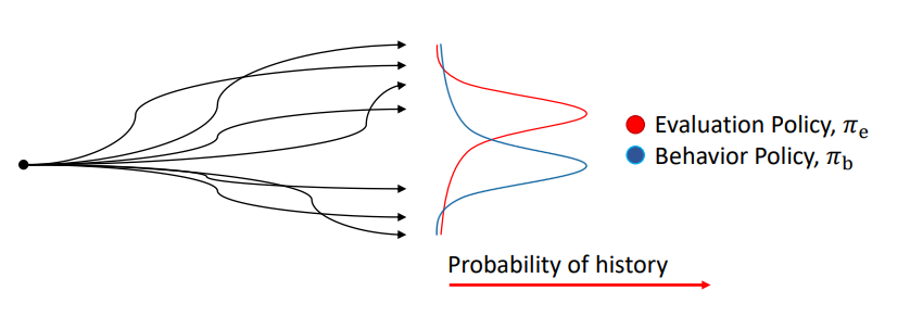
In the figure above, we have the episode rollouts and the probability of those episode. The performance of evaluation policy can be considered as importance-weighted return as described below. The weights are what changes when moving from behaviour to evaluation policy.
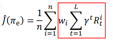
The episode corresponding to red peak in evaluation policy is what we will see a large number of times if we run the evaluation policy, but not when we run the behaviour policy. So, one idea is to estimate the performance of evaluation policy let us pretend that the episode if obtained often, by giving it higher weight.
We have X sampled from probability distribution p and Y from probability distribution q. We want to estimate E(f(X)), given samples Y.
Importance sampling estimator for E(f(X)), where X is sampled from probability p:
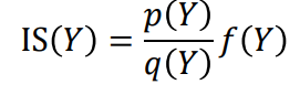
It can be proved that importance sampling gives an unbiased estimator of E(f(X)) under some assumptions.
Using the hoeffding’s inequality:
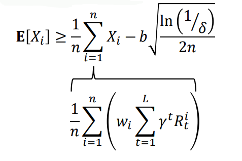
Here, Xi∈[0,b] and δ is the term we described earlier. Thus we can relate the expected value with sample estimator using importance sampling, in terms of the probability bound we have. There are far more stronger and complicated bounds than this that we can use like the Anderson and Massart’s or the CUT inequality but we won’t go in detail for those. Thus, we have bounded the performance of the target policy using samples for behaviour policy under some assumptions.We can use this method to decide whether we would update our policy, or return no solution found.
For more details and assumption on this method watch the talk by P.S Thomas.
I have covered some recent and contrasting methods on safe RL with the hope that this blog can serve as a footstep for you to apply your ideas in this domain. Yet another step to humanise AI.
References
- A Comprehensive Survey on Safe Reinforcement Learning
- Constrained Policy Optimization
- Safe, Multi-Agent, Reinforcement Learning for Autonomous Driving
- AI Safety Gridworlds
- Trial without Error: Towards Safe Reinforcement Learning via Human Intervention
- Safe Exploration in Continuous Action Spaces
- A great talk on safe RL by P.S Thomas
- OptLayer — Practical Constrained Optimization for Deep Reinforcement Learning in the Real World
- Virtuously Safe Reinforcement Learning
- Safe Reinforcement Learning via Formal Methods
- Eligibility Traces for Off-Policy Policy Evaluation
- P. S. Thomas. Safe Reinforcement Learning. PhD Thesis
This blog is based on papers cited in the reference and meant to be educational about the recent techniques in Safe Reinforcement Learning. All the credits for information goes to the respective authors. Thanks to Sohan Rudra and Anirban Santara for the fruitful discussions leading up to the blog.


Add comment